
Linear Regression is a type of statistical model where a linear relationship is established between one or more independent variables to a dependent variable. It’s one of the simplest types of predictive modeling.
Linear/multiple Regression models can be represented in the form of an equation
Y = A1X1 + A2X2 + … + AnXn + B
where Y is the dependent variable, Xn is the independent variables and An is the coefficient of Xn and B is the Intercept.
So, what is a coefficient? They are weights that are established to the independent variables based on the importance of the model. Let’s take an example of a simple linear regression that has one dependent variable Sales and an independent variable called Price. This can be represented in the form of an equation
Sales = A*Price + B
where A is Coefficient of Price. It explains the change in Sales when Price changes by 1 unit.
B is the intercept term which is also the prediction value you get when Price = 0
However, we must understand that there is always an error term associated with it. So, how do you reduce the error in the model?
The Line of Best Fit
The main purpose of the best fit line is to ensure that the predicted values are closer to our actual or the observed values. We must minimize the difference between the values predicted by us and the observed values. It’s termed as errors.
One technique to reduce the error is by using Ordinary Least Square (OLS). It tries to reduce the sum of squared errors ∑[Actual(Sales) – Predicted(Sales)]² by finding the best possible value of regression coefficient A.
This technique penalizes higher error value much more as compared to a smaller one so that there is a significant difference between making big errors and small errors. Thus it is easy to differentiate and select the best fit line.
You can also use other techniques like Generalized Least Square, Percentage Least Square, Total Least Squares, Least absolute deviation, and many more. However, OLS is easy to analyze and helps to differentiate and compute gradient descent. Interpretation of OLS is also much easier than other regression techniques.
Assumptions in Linear Regression
The following are some of the assumptions we make in a linear regression model:
- There exists a linear and additive relationship between the dependent and independent variables. By linear, it means that the change in the independent variable by 1 unit change in the dependent variable is constant. By additive, it refers to the effect of X on Y is independent of other variables.
- There is no multicollinearity (presence of correlation in independent variables). There must be no correlation between independent variables. If the variables are correlated, it becomes extremely difficult for the model to determine the true effect of IVs on DV.
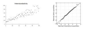
- The error terms must possess constant variance and an absence of it leads to Heteroskedasticity.
- The error terms must be uncorrelated. The presence of correlation in the error terms is called as autocorrelation. It drastically affects the regression coefficients and standard error values since they are based on the assumption of uncorrelated error terms.
- The dependent variable and the error terms must possess a normal distribution.
Tracking Violations of Assumptions
“How do I know if these assumptions are violated in my linear regression model ?”. Well, you have multiple ways to find out.
Residual vs. Fitted Values Plot
The plot between your residual and fitted values shouldn’t show any patterns. If you observe any curve or U shaped patterns, it means that there is a non-linearity in the data set. If you observe a funnel shape pattern it means that your data is suffering from heteroskedasticity- the error terms have non-constant variance.
Normality Q-Q Plot
It is used to determine the normal distribution of errors and uses a standardized value of residuals. This plot should show a straight line. If you find a curved, distorted line, then your residuals have a non-normal distribution.
Durbin Watson Statistic (DW)
This test is used to check autocorrelation. The value lies between 0 and 4. If the test value for DW =2, it means that there is no autocorrelation. If the value is between 0 and 2, it implies a positive autocorrelation, while a value greater an 2 implies negative autocorrelation.
Variance Inflation Factor (VIF)
This metric is also used to check multicollinearity. VIF of less than 4 implies that there is no multicollinearity but VIF >=10 suggests high multicollinearity. Alternatively, you can also look at the tolerance (1/VIF) value to determine correlation in independent variables.
Measuring the Performance of the Model
Do we have an evaluation metric to check the performance of the model?
R Square: It determines how much of the total variation in Y (dependent variable) is explained by the variation in X (independent variable). The value ranges from 0 to 1.
R Square = 1 – (Sum of Square Error/Sum of Square Total)
= 1 – ∑[YActual – YPredicted]²/ ∑[YActual – YMean]²
Let’s assume that you got a value of 0.432 as R Square for the above example. It means that only 43.2% of the variance in sales is explained by price. In other words, if you know the price, you’ll have 43.2% information to make an accurate prediction about the sales. Thus, the higher the value of R Square, the better the model (more things to consider).
Can R-Squared be negative? Yes, when your model doesn’t have an intercept. Without an intercept, the regression could do worse than the sample mean in terms of predicting the target variable. If the fit is actually worse than just fitting a horizontal line then R-square is negative.
When the number of independent variables in your model is more, it is best to consider adjusted R² than R² to determine model fit.
Adjusted R-Square: One problem with R² is that when the value increases proportionally to the number of variables increases. Irrespective of whether the new variable is actually adding information, the value increases. To overcome this problem, we use adjusted R² which doesn’t increase (stays the same or decrease) unless the newly added variable is truly useful.
Thus adjusted R-Square is a modified form of R-Square that has been adjusted for the number of predictors in the model. It incorporates the model’s degree of freedom. The adjusted R-Square only increases if the new term improves the model accuracy.
R² Adjusted = 1 – ((1-R²)(N-1))/(N – p – 1)
where, R² = Sample R square, p = Number of predictors, N = total sample size
F Statistics – It evaluates the overall significance of the model. It is the ratio of explained variance by the model by unexplained variance. Its value can range between zero and any large number. Naturally, higher the F statistics, better the model.
Other Metrics to evaluate
- Mean Square Error (MSE) – This is mean squared error. It tends to amplify the impact of outliers on the model’s accuracy. For example, if the actual y is 5 and predictive y is 25, the resultant MSE would be ∑(25-5)² = 400.
- Mean Absolute Error (MAE) – It’s the difference between the actual and predicted value. For the above example, the MAE would be ∑(25-5) = 20
- Root mean square error (RMSE) – It is interpreted as how far on an average is the residuals from zero. It nullifies the squared effect of MSE by square root and provides the result in original units as data. In the example, the RMSE would be √∑(25-5)² = 20. Note that the lower values of RMSE indicate better fit.