Theoretical Overview to Cluster Analysis

Cluster Analysis is a statistical technique that helps you divide your data points into a number of groups such that data points in the same groups are more similar to other data points in the same group than those in other groups. In simple word, it’s the process of organizing data into groups whose members are similar in some way.

It is considered to be the most important unsupervised learning technique (no dependent variable).

Applications

Some of the applications of cluster analysis are:

• Marketing: Business collects a large amount of data about its existing and potential customers. Clustering can be used to segment customers into groups and will help them in targeted marketing.
• Internet: Clustering can be used to group search results into a number of clusters based on the user’s query.
• Insurance: Identifying groups of motor insurance policyholders with some interesting characteristics.

It’s also used in Anomaly detection, Image Segmentation, Social Network Analysis etc.

Popular Clustering algorithms

Clustering algorithms can be classified into many types. However, they can be classified into two major types:

Hierarchical Clustering

A hierarchical clustering algorithm is based on the union between the two nearest clusters. There are two approaches to hierarchical clustering:

• Agglomerative method – starts with classifying all data points into separate clusters & then aggregating them as the distance decreases. The two ’closest’ (most similar) clusters are then combined and this is done repeatedly
  until all subjects are in one cluster. In the end, the optimum number of clusters is then chosen out of all cluster solutions.
• Divisive methods, in which all the data points start in the same cluster and the above strategy is applied in reverse until every subject is in a separate cluster. Also, the choice of the distance function is subjective.

Note that Agglomerative methods are used more often than divisive methods. These models are very easy to interpret but lack the scalability to handle large datasets.

In this article, I will explain how hierarchical clustering can be done using Agglomerative Method. The results of hierarchical clustering can be interpreted using a dendrogram.

Distance

An important component of a clustering algorithm is the distance measure between data points. The decision of merging two clusters is taken on the basis of the closeness of these clusters (distance). There are multiple metrics for deciding the closeness of two clusters :

• Euclidean distance: ||a-b||₂ = √(Σ(a_i-b_i))
• Squared Euclidean distance: ||a-b||₂² = Σ((a_i-b_i)²)
• Manhattan distance: ||a-b||₁ = Σ|a_i-b_i|
• Maximum distance:||a-b||_INFINITY = max_i|a_i-b_i|
• Mahalanobis distance: √((a-b)^T S^-1 (-b))   {where, s : covariance matrix}

We use these distance metrics based on the methodology. Under the Agglomerative method, there are also a number of different methods used to determine which clusters should be joined at each stage. Some of the main methods are summarised below:

• Nearest neighbor method (single linkage method): In this method, the distance between two clusters is defined to be the distance between the two closest members, or neighbors. This method is relatively simple but is often criticised because it doesn’t take account of cluster structure and can result in a problem called chaining whereby clusters end up being long and straggly.
• Furthest neighbor method (complete linkage method): In this case, the distance between two clusters is defined to be the maximum distance between members — i.e. the distance between the two subjects that are furthest apart. It’s also sensitive to outliers.
• Average (between groups) linkage method (sometimes referred to as UPGMA): The distance between two clusters is calculated as the average distance between all pairs of subjects in the two clusters.
• Centroid method: The centroid (mean value for each variable) of each cluster is calculated and the distance between centroids is used. Clusters whose centroids are closest together are merged.
• Ward’s method: In this method, all possible pairs of clusters are combined and the sum of the squared distances within each cluster is calculated. This is then summed over all clusters. The combination that gives the lowest sum of squares is chosen.

Selecting the Number of Clusters

Once the cluster analysis has been carried out, we need to select the ’best’ cluster solution. When carrying out a hierarchical cluster analysis, the process can be represented on a diagram known as a dendrogram.

A dendrogram illustrates which clusters have been joined at each stage of the analysis and the distance between clusters at the time of joining. If there is a large jump in the distance between clusters from one stage to another then this suggests that at one stage clusters that are relatively close together were joined whereas, at the following stage, the clusters that were joined were relatively far apart. This implies that the optimum number of clusters may be the number present just before that large jump in distance.

Thus, the best choice of the no. of clusters is the no. of vertical lines in the dendrogram cut by a horizontal line that can transverse the maximum distance vertically without intersecting a cluster.

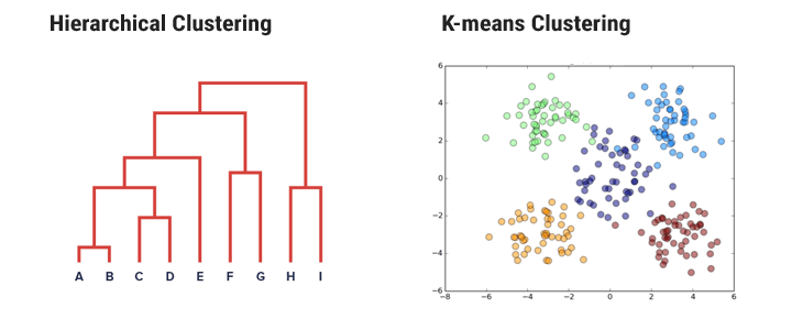
Non-hierarchical or k-means clustering methods

K means is an iterative clustering algorithm that aims to find local maxima in each iteration. The notion of similarity is derived by the closeness of a data point to the centroid of the clusters.  In this model, the no. of clusters required at the end have to be mentioned beforehand, which means that you need to have prior knowledge of the dataset. These models run iteratively to find the local optima.

Non-hierarchical cluster analysis tends to be used when large data sets are involved. However, it is difficult to know how many clusters you are likely to have and therefore the analysis. It can be very sensitive to the choice of initial cluster centers.

Methodology:

1. Choose initial cluster centers (essentially this is a set of observations that are far apart – each subject forms a cluster of one and its center is the value of the variables for that subject).
2. Assign each subject to its ’nearest’ cluster, defined in terms of the distance to the centroid.
3. Find the centroids of the clusters that have been formed
4. Re-calculate the distance from each subject to each centroid and move observations that
   are not in the cluster that they are closest to.
5. Continue until the centroids remain relatively stable i.e when there will be no further switching of data points between two clusters for two successive repeats. It will mark the termination of the algorithm if not explicitly mentioned.

Best Approach: First use a hierarchical clustering to generate a complete set of cluster solutions and establish the appropriate number of clusters. Then, you use a k-means (nonhierarchical) method.

Other Clustering algorithms

All though K-means and Hierarchical clustering are the popular methods, there are some other clustering algorithms like Fuzzy C-Means and Mixture of Gaussians.

Fuzzy C-Means Clustering

Fuzzy C-means (FCM) is a technique in which a dataset is grouped into n clusters with every data point in the dataset belonging to every cluster to a certain degree (an overlapping clustering algorithm). For example, a certain data point that lies close to the center of a cluster will have a high degree of belonging or membership to that cluster and another data point that lies far away from the center of a cluster will have a low degree of belonging or membership to that cluster.

It starts with an initial guess for the cluster centers that is intended to mark the mean location of each cluster. The algorithm then assigns every data point a membership grade for each cluster. By iteratively updating the cluster centers and the membership grades for each data point, it iteratively moves the cluster centers to the right location within a data set.

The advantage with this algorithm is that it gives the best result for overlapped data set and is comparatively better then k-means algorithm. However, we have to specify the number of clusters beforehand.

Mixture of Gaussians

It’s a probability clustering algorithm. Each cluster can be mathematically represented by a parametric distribution, like a Gaussian (continuous) or a Poisson (discrete). The entire data set is therefore modeled by a mixture of these distributions.

Gaussian mixture models (GMMs) assumes all the data points are generated from a mixture of a finite number of Gaussian distributions with unknown parameters. It assigns each observation to a cluster by maximizing the posterior probability that a data point belongs to its assigned cluster. The method of assigning a data point to exactly one cluster is called hard clustering.

GMMs have been used for feature extraction from speech data, and have also been used extensively in object tracking of multiple objects, where the number of mixture components and their means predict object locations at each frame in a video sequence.

If you like the article, do share your views in the comment section below