
Definition: Logistic regression is a statistical method that helps analyze a dataset in which there are one or more independent variables and has a dependent variable that is binary or dichotomous (there are only two possible outcomes). It was developed by statistician David Cox in 1958.
The dependent variable can only take two values i.e. 0 or 1, YES or NO, Default or No Default etc. The independent factors or variables can be categorical or numerical variables.
Application: Logistic regression is used to predict a binary outcome. A Credit card company can build a model, decide whether to issue a credit card to a customer or not based on various parameters. The model will help the company identify whether the customer is going to “Default” or “Not Default” on this credit card (also called as Default Propensity Modelling).
Similarly, in the healthcare sector, it can be used to predict the outcome for a disease (whether the subject suffers from a particular disease or not) based on various variables such as body temperature, pressure, age etc.
The model is:
logit (p) = a + b1X1 + … + bnXn,
where logit (p) = ln{p/(1- p)}
and n is the expected probability of an event and ln is the natural logarithm.
Training the Model (using R)
The dataset is called Titanic and contains 4 independent variables – Age of the Passenger, Gender of the Passenger, Class of Travel (1st, 2nd, and 3rd Class) and Fare. The dependent variable is Survival (whether the passenger survived or not)
The following code was executed in R to create a simple GLM model for the dataset:
titanic<- read.csv("titanic.csv")
titanic$Class <- as.factor(titanic$Class)
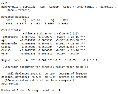
titanic.glm <- glm(Survival~Age+Gender+Class+Fare, data=titanic, family="binomial")
summary(titanic.glm)
The results of the model are summarised below:
Interpreting the Model
The coefficient associated with the variable Gender is -2.4935, so the odds of surviving for a Male is exp(-2.4935)= 0.082 times that of a woman of the same age, class, and fare.
The coefficient for age = -0.034313 which is interpreted as the expected change in log odds for a one-unit increase in the age. The odds ratio can be calculated by using exponential function (exp(-0.034)) to get value = 0.9662689 which means we expect to see about 3.37% decrease in the odds of survival, for a one-unit increase in age.
Measuring the Performance of the Model
1. AIC (Akaike Information Criteria): It is a measure of both how well the model fits the data and how complex the model is. It is the measure of fit which penalizes model for the number of model coefficients. It helps you find the best-fitting model that uses the fewest variables and thus we prefer a model with minimum AIC. But it won’t say anything about absolute quality.
AIC = -2(log-likelihood) + 2K
Where:
- K is the number of variables in the model plus the intercept.
- Log-likelihood is a measure of model fit. The higher the number, the better the fit.
2. Null Deviance and Residual Deviance: The null deviance shows how well the response variable is predicted by a model that includes only the intercept. Lower the value, better the model. Residual deviance indicates the response predicted by a model on adding independent variables. Lower the value, better the model.
3. Fisher’s scoring algorithm: It is a derivative of Newton’s method for solving maximum likelihood problems numerically.
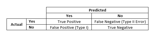
4. Confusion Matrix: It’s nothing but the tabular representation of the actual and predicted values which will help assess the performance of a classification model.
 Terminologies
- True positives (TP): These are cases in which we predicted yes, and the actual result was also yes.
- True negatives (TN): We predicted no, and the actual result was also no
- False positives (FP): We predicted yes, but the actual was no. (Also known as a “Type I error.”)
- False negatives (FN): We predicted no, but the actual was yes. (Also known as a “Type II error.”)
Some important metrics from the Confusion Matrix
- Accuracy of the Model = (True Positives + True Negatives) / Total Number of Observations
- Misclassification Rate or Error Rate = (False Positives + False Negatives) / Total Number of Observations = 1 – Accuracy
- True Positive Rate (also known as “Sensitivity” or “Recall”) = TP/(TP+FN)
- False Negative Rate = FN/(TP+FN) = 1-Sensitivity
- True Negative Rate (also known as “Specificity”) = TN/(TN+FP)
- False Positive Rate = 1 – Specificity = FP/(TN+FP)
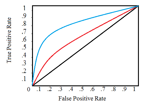
5. Receiver Operating Characteristic (ROC) Curve helps visualize the model’s performance. It is a plot of the true positive rate (sensitivity) against the false positive rate (1- Specificity). The area under the curve (AUC) (also known as the index of accuracy (A) or concordance index), is a performance metric for ROC curve. Higher the area under the curve, better the prediction power of the model. A perfect test has an area under the ROC curve as 1. The worst model (useless model) will have the AUC as 0.5.
The closer the graph is to the top and left-hand borders, the more accurate the model is. Likewise, the closer the graph to the diagonal, the less accurate the test.
Leave a Reply