Introduction to ANOVA

ANOVA (Analysis of Variance) is a statistical technique used to check if the means of two or more groups are significantly different from each other. It may seem odd that it’s called “Analysis of Variance” rather than “Analysis of Means”. However, the name is appropriate since we make inferences about means by analyzing variance.

If we are only comparing two means, ANOVA will produce the same results as the t-test for independent samples (if we are comparing two different groups) or the t-test for dependent samples (if we are comparing two variables in one set of observations).

Then why not use multiple t-tests? If you were to conduct multiple t-tests for comparing more than two samples, it will have a compounded effect on the error rate of the result.

Application: Consider a scenario where you get a sample of the annual income of employees from three different geographies. You might want to compare if there is a difference in the average income of employees based on geographies. In this case, you would use ANOVA to compare the average income.

Another application of ANOVA can be found in the medical sector. In order to understand a reliable treatment method for a disease, multiple test groups (based on cure methodology) would be created. They would try to measure the number of days it takes to cure for each test group. Here, ANOVA can be used to prove/disprove if all the medication treatments were equally effective or not.

Assumptions

The following are the assumptions in ANOVA:

• Each group sample is drawn from a normally distributed population
• The populations have a common variance
• The samples are drawn independently of each other
• Within each sample, the observations are sampled randomly and independently of each other

Terminologies

Grand Mean: Mean is a simple or arithmetic average of a range of values. In ANOVA, we use two types of means – the grand mean (mean of the entire sample) and group sample means (mean of each individual groups).

Hypothesis: A hypothesis is a statement which is suggested as a possible explanation for a particular situation or condition, but which has not yet been proved to be correct. In the case of ANOVA, we have a Null Hypothesis and an Alternate Hypothesis.

• Null hypothesis – All sample means are equal, or they don’t have any significant difference.
• Alternate hypothesis – At least one of the sample means is different from the rest of the sample means.

Note that we still can’t tell which group is specifically different from rest of the others.

Between-Group Variability (Mean Square Effect): It refers to variations between the distributions of individual groups as the values within each group are different. To calculate the Mean Square effect, we look at each sample to calculate the difference between its mean and the grand mean.

• Sum of Square for between-group variability (SS_B): It’s the aggregate of squared differences between the sample mean and the grand mean.
• Mean sum of Square for between-group variability (MS_B): It’s calculated by dividing the Sum of Square (between-group variability) and the degrees of freedom (number of sample means – 1)

Within-Group Variability (Mean Square Effect): It refers to variations caused by differences within individual groups as not all the values within each group are the same. Each sample is considered independently, no interaction between samples is involved and the variability between the individual points in the sample is calculated.

• Sum of Square for within-group variability (SS_W): It is the aggregate of squared deviation of each value from its respective sample mean.
• Mean sum of Square for within-group variability (MS_W): It’s calculated by dividing the Sum of Square (within-group variability) and the degrees of freedom (the sum of the individual degrees of freedom for each sample). Since each sample has degrees of freedom equal to one less than their sample sizes, and there are k samples, the total degrees of freedom is k less than the total sample size: df = N – k.

Total Variation: It is the sum of the squares of the differences of each mean with the grand mean which is also the sum of SS_B and SS_W.

The whole idea behind the analysis of variance is to compare the ratio of between-group variance to within-group variance. If the variance caused by the interaction between the samples is much larger when compared to the variance that appears within each group, then it is because the means aren’t the same.

F test statistic: It measures if the means of different samples are significantly different or not. It’s calculated by dividing MS_B and MS_W. Lower the F-Ratio, more similar are the sample means. In that case, we cannot reject the null hypothesis.

The F-statistic calculated here is compared with the F-critical value for making a conclusion. If the value of the calculated F-statistic is more than the F-critical value (for a specific α/significance level), then we reject the null hypothesis.

Summary Table:

Variability	Sum of Square	Degrees of Freedom	Mean Square	F Statistic
Between	SSB	k – 1	SSB/(k-1)	MSB/MSW
Within	SSW	N – k	SSW/(N – k)
Total	SSB + SSW	N – 1

Types of ANOVA Test for Univariate Analysis

There are commonly two types of ANOVA tests for univariate analysis – One-Way ANOVA and Two-Way ANOVA. One-way ANOVA is used when we are interested in studying the effect of one independent variable (IDV)/factor on a population, whereas Two-way ANOVA is used for studying the effects of two factors on a population at the same time.

One Way ANOVA in Excel 2013

The following steps will help you carry out ANOVA in Microsoft Excel 2013:

• Step 1: Input your data into rows and columns in Excel. If you have three groups as shown in the example, spread the data into three columns.
• Step 2: Click the “Data” tab on the ribbon and then click “Data Analysis”. If you don’t see Data Analysis, load the ‘Data Analysis Toolpak’ add-in. It can be loaded by clicking “Options: in the File Menu. Then click on “Add-Ins” and you will be able to manage your Add-Ins.
• Step 3: Click on “ANOVA Single Factor” and then click “OK”. Then, Input the Range of values and set the Alpha value (default = 0.05, 95% confidence). Click “Ok” to see the output.

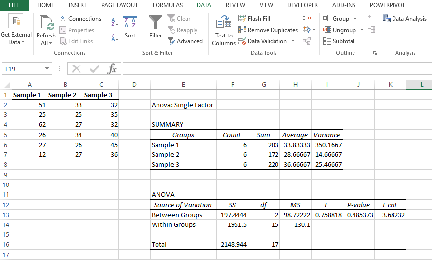
From the Excel Output above, we see that p-value = 0.485 > 0.05, and so we can reject the null hypothesis and conclude there is a significant difference between the means of the four samples. The F-value is also smaller than the f critical value.

Two Way ANOVA in Excel 2013

The steps are similar to One-way ANOVA in Microsoft Excel 2013:

• Step 1: Input your data into rows and columns in Excel as shown in the screenshot below.
• Step 2: Click the “Data” tab on the ribbon and then click “Data Analysis”. If you don’t see Data Analysis, load the ‘Data Analysis Toolpak’ add-in.
• Step 3: Click on “ANOVA two factor with replication” and then click “OK”. Then, Input the Range of values and set the Alpha value (default = 0.05, 95% confidence). Click “Ok” to see the output.

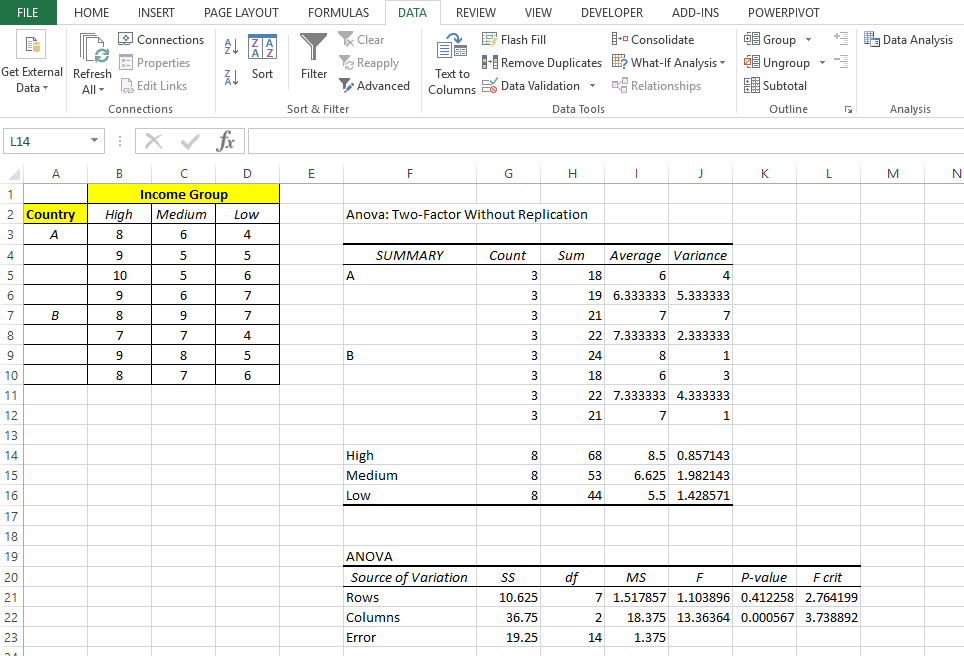
From the excel output above, we can conclude that for Row-wise (Country wise), there is a difference in the means. However, for column-wise (Income Levels), we failed to reject the null hypothesis (p < 0.05) and hence there is no difference in the means.